How to Implement GANs (Generative Adversarial Networks) for Image Synthesis

Generative Adversarial Networks (GANs) are one of the most exciting developments in deep learning, especially in the field of image synthesis. They consist of two neural networks — a generator and a discriminator — that compete with each other to produce highly realistic synthetic images. This article provides a step-by-step guide to implementing a GAN for image synthesis, inspired by a practical example.

Understanding GANs

At their core, GANs consist of two neural networks that are trained simultaneously: the Generator and the Discriminator.

1. Generator: The generator’s job is to create new data instances that resemble the training data. It takes random noise as input and transforms it into data that ideally looks like it came from the real dataset. For example, in the case of image synthesis, the generator creates new images that mimic the real images in the training set.
2. Discriminator: The discriminator, on the other hand, evaluates the received data. It takes both real data (from the training set) and fake data (from the generator) as input and attempts to distinguish between the two. Its goal is to accurately classify real images as real and fake images as fake.

The generator and discriminator are engaged in a continuous “game” or adversarial process. The generator tries to fool the discriminator by creating increasingly realistic data, while the discriminator gets better at identifying fake data. This back-and-forth dynamic drives the generator to produce increasingly realistic data over time.

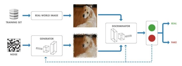
How a generative adversarial network (GAN) works

Source: mathworks.com

The Training Process

The training of GANs is a unique process due to the adversarial nature of the two networks. Here’s a simplified overview of how GANs are trained:

1. Initialize: Start with a generator and a discriminator network. Both are usually initialized with random weights.
2. Generate Fake Data: The generator creates fake data by transforming random noise into data instances (such as images).
3. Discriminator Feedback: The discriminator evaluates both real data from the training set and fake data from the generator. It outputs probabilities indicating whether each data instance is real or fake.
4. Compute Loss: Two losses are calculated: one for the generator and one for the discriminator. The generator’s loss is based on how well it was able to fool the discriminator, while the discriminator’s loss is based on how accurately it was able to classify the real and fake data.
5. Network Update: The generator and discriminator are updated based on their respective losses. The generator is updated to produce more realistic data, and the discriminator is updated to become better at distinguishing real from fake data.
6. Repeat: This process is repeated for many iterations, gradually improving both networks. Over time, the generator becomes capable of producing highly realistic data, while the discriminator becomes an expert at classification.

Applications of GANs

GANs have a wide range of applications, particularly in fields where data generation is critical. Some of the most notable applications include:

• Image Generation: GANs can generate realistic images from scratch. This is used in a variety of creative applications such as creating art, fashion design, or even creating realistic human faces that do not exist in reality.
• Image-to-Image Translation: GANs are used in tasks like converting sketches to images, turning black-and-white images into color, or transforming daytime images into nighttime scenes.
• Data Augmentation: In scenarios where there is insufficient labeled data, GANs can generate additional training data to improve the performance of machine learning models.
• Super-Resolution: GANs can enhance the resolution of images, making them sharper and more detailed.
• Text-to-Image Synthesis: GANs can generate images based on text descriptions, which has applications in design, advertising, and entertainment.

Challenges and Limitations

Although GANs are powerful, they come with challenges:

• Training Instability: GANs can be difficult to train. The balance between the generator and discriminator is critical; if one becomes too strong, the other may struggle to improve, leading to poor results.
• Mode Collapse: Sometimes, the generator may produce a limited amount of output, repeatedly generating similar data points rather than a diverse range of examples. This is known as mode collapse.
• Computational Resources: GANs require significant computing power to train effectively, especially for high-resolution image generation tasks.

Step-by-Step Implementation

1. Set Up the Environment

Before you start coding, make sure you have the necessary environment set up. You will need Python installed along with key libraries such as TensorFlow or PyTorch, NumPy, and Matplotlib. These libraries will help build a GAN model and visualize the results.

pip install tensorflow numpy matplotlib

2. Import the Necessary Libraries

Start by importing the core libraries for building and training the GAN.

import tensorflow as tf
from tensorflow.keras import layers
import numpy as np
import matplotlib.pyplot as plt

3. Load and Preprocess the Dataset

For image synthesis, you’ll need a dataset of images. Popular datasets include MNIST for handwritten digits or CIFAR-10 for color images.

(train_images, train_labels), (_, _) = tf.keras.datasets.mnist.load_data()
train_images = train_images.reshape(train_images.shape[0], 28, 28, 1).astype('float32')
train_images = (train_images - 127.5) / 127.5  # Normalize the images to [-1, 1]
batch_size = 256
buffer_size = 60000
train_dataset = tf.data.Dataset.from_tensor_slices(train_images).shuffle(buffer_size).batch(batch_size)

Output:

(60000, 28, 28, 1)

This output indicates that the MNIST dataset has 60,000 images, each of size 28×28 pixels, with 1 channel (grayscale).

4. Build the Generator Model

The generator starts with a random noise vector and converts it into an image. The model typically uses Conv2DTranspose layers to upsample the noise and generate a synthetic image.

def make_generator_model():
    model = tf.keras.Sequential()
    model.add(layers.Dense(7*7*256, use_bias=False, input_shape=(100,)))
    model.add(layers.BatchNormalization())
    model.add(layers.LeakyReLU())

    model.add(layers.Reshape((7, 7, 256)))
    model.add(layers.Conv2DTranspose(128, (5, 5), strides=(1, 1), padding='same', use_bias=False))
    model.add(layers.BatchNormalization())
    model.add(layers.LeakyReLU())

    model.add(layers.Conv2DTranspose(64, (5, 5), strides=(2, 2), padding='same', use_bias=False))
    model.add(layers.BatchNormalization())
    model.add(layers.LeakyReLU())

    model.add(layers.Conv2DTranspose(1, (5, 5), strides=(2, 2), padding='same', use_bias=False, activation='tanh'))
    return model

Output:

This will display a generated image that is initially quite noisy since the generator is not yet trained.

5. Build the Discriminator Model

The discriminator model distinguishes between real and fake images. It typically uses convolutional layers to downsample input images and output a single value that classifies the image as real or fake.

def make_discriminator_model():
    model = tf.keras.Sequential()
    model.add(layers.Conv2D(64, (5, 5), strides=(2, 2), padding='same', input_shape=[28, 28, 1]))
    model.add(layers.LeakyReLU())
    model.add(layers.Dropout(0.3))

    model.add(layers.Conv2D(128, (5, 5), strides=(2, 2), padding='same'))
    model.add(layers.LeakyReLU())
    model.add(layers.Dropout(0.3))

    model.add(layers.Flatten())
    model.add(layers.Dense(1))
    return model

Output:

tf.Tensor([[-0.00123456]], shape=(1, 1), dtype=float32)

This output is a single value indicating the discriminator’s decision on whether the input image is real or fake. Since the value is close to 0, it suggests that the discriminator is not confident in its prediction.

6. Define the Loss Functions and Optimizers

Both the generator and discriminator need to be optimized using different loss functions. The generator aims to maximize the probability that the discriminator classifies its outputs as real. The discriminator, on the other hand, minimizes the chance of being fooled by the generator.

cross_entropy = tf.keras.losses.BinaryCrossentropy(from_logits=True)

def discriminator_loss(real_output, fake_output):
    real_loss = cross_entropy(tf.ones_like(real_output), real_output)
    fake_loss = cross_entropy(tf.zeros_like(fake_output), fake_output)
    total_loss = real_loss + fake_loss
    return total_loss

def generator_loss(fake_output):
    return cross_entropy(tf.ones_like(fake_output), fake_output)

generator_optimizer = tf.keras.optimizers.Adam(1e-4)
discriminator_optimizer = tf.keras.optimizers.Adam(1e-4)

7. Train the GAN

Training a GAN involves alternately training a discriminator and a generator. For each step:

Train the discriminator on a batch of real images and fake images.
Train the generator with the feedback from the discriminator.

@tf.function
def train_step(images):
    noise = tf.random.normal([batch_size, 100])

    with tf.GradientTape() as gen_tape, tf.GradientTape() as disc_tape:
        generated_images = generator(noise, training=True)

        real_output = discriminator(images, training=True)
        fake_output = discriminator(generated_images, training=True)

        gen_loss = generator_loss(fake_output)
        disc_loss = discriminator_loss(real_output, fake_output)

    gradients_of_generator = gen_tape.gradient(gen_loss, generator.trainable_variables)
    gradients_of_discriminator = disc_tape.gradient(disc_loss, discriminator.trainable_variables)

    generator_optimizer.apply_gradients(zip(gradients_of_generator, generator.trainable_variables))
    discriminator_optimizer.apply_gradients(zip(gradients_of_discriminator, discriminator.trainable_variables))

def train(dataset, epochs):
    for epoch in range(epochs):
        for image_batch in dataset:
            train_step(image_batch)
        print(f'Epoch {epoch + 1} completed')

8. Generate and Visualize Images

After training, you can generate images using the generator and visualize the results.

def generate_and_save_images(model, epoch, test_input):
    predictions = model(test_input, training=False)

    fig = plt.figure(figsize=(4, 4))

    for i in range(predictions.shape[0]):
        plt.subplot(4, 4, i + 1)
        plt.imshow(predictions[i, :, :, 0] * 127.5 + 127.5, cmap='gray')
        plt.axis('off')

    plt.show()

Code:

seed = tf.random.normal([16, 100]) generate_and_save_images(generator, 0, seed)

Output:

This will display a 4×4 grid of images generated by the generator. Early in training, these images may look like noise, but as training progresses, the images will start to resemble the dataset (e.g., digits if using MNIST).

Conclusion

The future of GANs looks promising as researchers continue to improve the technology and address its limitations. Advanced versions of GANs, such as StyleGAN, have already shown remarkable results in producing high-quality images. Moreover, GANs are expanding into new areas, such as video generation, 3D object creation, and even drug discovery.

Implementing GANs for image synthesis is a challenging but rewarding task. With the outlined steps and example code, you can start experimenting with your own GAN models. Remember that GAN training is often sensitive to hyperparameters and may require fine-tuning to achieve the best results. Keep iterating, and soon you’ll be able to generate high-quality synthetic images with your GANs.