Diabetes is a disease where time matters. Regular ophthalmological examination and analyses of retinal images can help in early detection and treatment. For patients suffering from moderate to severe stages, it is necessary to conduct ophthalmological examinations with high frequency for the presence of progress in diabetic retinopathy. This is not always possible, due to the high number of patients and lack of doctors.
And that’s another sphere where AI could be helpful. Specialized retinal image analysis systems developed using modern artificial intelligence methods can help an ophthalmologist simplify the task of monitoring the condition of the patient’s fundus.
The purpose of this article is to share the experience of implementing a system for the detection and classification of diabetic retinopathy using AI tools.
Background
As is well known, diabetes mellitus and its complications are one of the most serious medical, social, and economic problems of modern healthcare. Diabetic retinopathy is a complication of diabetes mellitus that affects the blood vessels of the retina of the eye. Retinopathy begins completely asymptomatically, and the patient does not notice it for a long time. Loss or decrease in visual acuity signals an irreversible complication process. An effective system for the detection and treatment of diabetic retinopathy, including healthcare app development solutions, can significantly reduce the risk of blindness and the associated economic costs. Modern ophthalmology has the knowledge to combat this complication of diabetes, including laser coagulation and vitrectomy. The number of diabetic patients is growing, and diabetic retinopathy is one of the most severe complications, often leading to blindness. Laser treatment of one patient is 12 times cheaper than social benefits for one blind person. Also, in practice, there are cases when the patient does not even suspect the presence of diabetes mellitus for a long time, but the detection of diabetic retinopathy may indicate the presence of an underlying disease. According to the World Health Organization (WHO), there are 5 stages of the disease:
0 – No DR
1 – Mild
2 – Moderate
3 – Severe
4 – Proliferative DR
According to WHO, there are major problems: microaneurysms are local dilations of retinal vessels associated with excessive permeability in the macular area, leading to macular edema; hemorrhages; “hard” exudates; “soft” exudates retinal edema. Some of these problems are shown in the figure in a patient suffering from stage 4 of the Diabetic retinopathy:
Thus, the task was set to create for a medical clinic a software product for classifying diabetic retinopathy into 4 stages. The main work related to achieving the goal consisted of the following stages: creation of a research plan, search for a suitable data set for training and validation, research and experiments with existing neural network architectures, implementation of system code based on the selected neural network, model training, analysis of results on images by the hospital.
Challenges and Resolutions
The first problem that had to be solved in the course of solving this engineering problem was where to get a training sample? During the study of this problem, many sources were analyzed for the availability of ready-made datasets with fundus images. A brief overview of ready-made data sets on the Internet distributed under a free licence is shown in the table:
Since 2015 on the resource kaggle.com an extensive dataset is available for download, consisting of 35,126 images for network training, and 53,576 images for validation of results. As a result, this particular dataset was used for training in this project.
The second problem that arises for every ML engineer who is solving image classification problem – to choose a neural network type from a large set of existing ones. Next, is presented to your attention the quality formula of the above – mentioned convolutional neural networks, depending on such characteristics as the width, depth and resolution of the network:
The formula shows that as the network depth increases, the accuracy of the network increases in direct proportion, which is a good sign, but there is a problem with gradient attenuation. This problem is described in detail in the article “Performance Comparison of CNN Models Using Gradient Flow Analysis ” by Saul-Hyun Noah from 2021. The next way to increase the accuracy of the network is the width. It can be seen from the formula that the larger the width of the network, the more accurate the network is. At the same time, there is a quadratic dependence of the network on its width. Similarly, to increase the accuracy of the network, the resolution is. That is, the higher the input resolution, the more accurate the network is. At the same time, again, the formula shows that there is a quadratic dependence of the network on the input resolution.
The authors of the article [EfficientNet: Rethinking Model Scaling for Convolutional Neural Networks] propose a new composite scaling method that uniformly scales depth/width/resolution with fixed proportions between them. As a result, the authors receive a new class of models called Efficient Net, which already contains the most optimal starting weight coefficients. There are several subsets of these architectures of a given network from B0 to B7, depending on the required accuracy. The scheme of operation of these networks is shown in the figure, in comparison with other networks. It was this network that was chosen to solve the task. The comparison of the EfficientNet with others networks is shown on the picture:
The next important step was to build a model based on the Efficient Net network discussed above. Let’s take a step-by-step look at what happens in each line:
Input Layer:
- input_layer = tf.keras.layers.Input(shape=(*self._img_size_list, 3)):
This line creates an input layer for the model that expects images of the shape specified by a list defining the height and width of the images. The 3 indicates that the images are expected to have 3 colour channels (RGB).
Data Augmentation:
- augmented = self._data_augmentation(input_layer):
Applies data augmentation to the input images using a method defined elsewhere in the class. Data augmentation is a technique used to increase the diversity of the training data without actually collecting new data, by applying random transformations like rotation, scaling, etc.
Base Model:
- base_model = self.EFNS[ef](input_shape=(*self._img_size_list, 3), weights=’imagenet’, include_top=False):
Loads one of the EfficientNet models as the base model with pre-trained weights from ImageNet. Second argument indicates that the top layer of the network, typically used for classification, is not included, allowing for custom layers to be added.
Feature Extraction:
- features = base_model(augmented):
Passes the augmented images through the base model to extract features.
Pooling Layer:
- pooled_features = tf.keras.layers.GlobalAveragePooling2D()(features):
Applies global average pooling to the features, which reduces the spatial dimensions (height and width) to a single value per channel. This is useful to condense the information into a form suitable for classification.
Output Layer:
- classifier_output = tf.keras.layers.Dense(self._num_classes, activation=’softmax’)( pooled_features):
Adds a fully connected layer with a number of units equal to the number of classes In the current case this number equals the number of stages of the disease. The softmax activation function is used to calculate the probability distribution over the classes.
Model Creation:
- model = tf.keras.Model(inputs=input_layer, outputs=classifier_output):
Creates the Keras model with the defined input and output layers.
Compilation:
- optimizer = tf.keras.optimizers.Adam(learning_rate=0.001):
Initialises the Adam optimizer with a learning rate of 0.001.
- model.compile(optimizer=optimizer, loss=’sparse_categorical_crossentropy’, metrics=[‘accuracy’]):
Compiles the model with the Adam optimizer, using sparse_categorical_crossentropy as the loss function (commonly used for multi-class classification tasks), and tracking the accuracy metric.
Then it was necessary to train the model using training data. In total, 5 stages of training were conducted:
- Preparing the train dataset:
- self._get_training_dataset(files_train):
This method is to return a preprocessed dataset ready for training, using the training files.
- Setting the required number of epochs:
- epochs=self.epoch_count:
The number of times for the dataset to pass through the neural network in the forward and reverse directions
- Callbacks for viewing internal states and statistics:
- sv:
Model checkpoint callback to save the model at certain intervals.
- self._get_lr_callback(self.batch_size):
Adjusts the learning rate based on the batch size or other criteria.
- logger:
Logs epoch results to a CSV file.
- Number of steps per epoch:
- steps_per_epoch:
The number of batches of samples to execute during each epoch, which is the total number of training items divided by the batch size, and then divided by the number of replicas (if training is distributed across multiple devices).
- Preparing the validation dataset:
- validation_data:
Getting the loss and quality metrics after finishing each epoch.
- Number of steps per epoch for validation:
- validation_steps:
Similar to steps_per_epoch, but for the validation dataset.
- Progress bar during training:
- verbose:
This controls the verbosity of the output during training (e.g., whether to show a progress bar).
Model training
The training takes place in 5 stages (folds). Each stage of the sampling data randomly shuffles the initial values of the experiments. A fifth part of them is used to verify the correctness of training (validation set in TensorFlow terms), the remaining data is used to train the model.
Thus, from stage to stage, the training data may differ, as a result, it will be possible to choose the weight coefficients with the best results.
The TF library allows You to determine the success of model training by storing critical data at each stage of training. The absolute value of losses (loss) and accuracy of predictions (accuracy) are used as such data.
Experimentally, it was found that the best result in training is given by the number of training epochs equal to 25. The NVIDIA RTX 3060 GPU with 12 GB of video memory allows parallel processing of a packet from the source data.
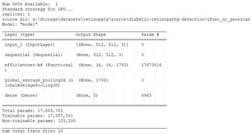
Model data before starting training:
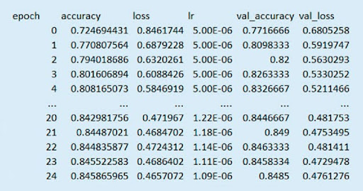
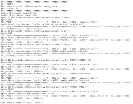
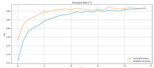
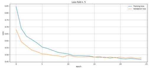
As a result of training, the model of the fifth stage can be considered the best from the point of view of real use, since the loss and accuracy graphs coincide more often than at other stages of training. For this reason, below are visualisations of model training for stage five. The fifth training cycle takes 72 900s (20 hours 15 minutes 0 seconds). The learning error matrices are shown in the figure:
The history of events at the fifth stage of training:
Accuracy of training in the fifth stage of training:
The amount of losses at the fifth stage of training:
It can be seen from the training results that the trained neural network is able to determine the degree of diabetic retinopathy with a probability of 85 percent.
Testing and experiments
After testing the model, the following indicators were obtained:
The model is very effective at predicting class 0(no retinopathy) but has difficulty with the first stage of the disease, and it performs moderately for the other classes. The overall accuracy is high, but the low recall for some classes indicates that the model may be missing a significant number of positive cases for those classes. But this situation is normal, since the detection of the first stage of the disease cannot always be detected with certainty, even from fundus photographs, and in this case other tests and techniques are used in medicine.
The next step is to lead the experiment and examine the model in practice for a patient from a real medical clinic. During the development of this software, work was conducted with colleagues from a medical clinic, which provided this photograph of an anonymous patient. It was known in advance that the patient suffered from the second stage of retinopathy. The photograph has a non-standard resolution – 1750 x 1462 pixels, as well as a non-standard shape, this is explained by the desire to cover as much as possible the entire area of the patient’s fundus and is determined by the peculiarities of the work of each ophthalmologist:
Well, let’s look at the result of the experiment:
As can be seen from the results of the software, despite the non-standard parameters of fundus photography, the second stage of retinopathy was successfully confirmed.
Conclusion
This article showed how to build an application based on neural networks. The key stages were considered, such as – justification of the choice of a ready-made neural network, creating the neural network based on an already existing deep neural network, training of the network, quality assessment, etc.
The research conducted in this project has shown that deep learning neural networks are able to effectively determine the degree of the disease. The weighted average f1 score of pathology detection of 82% makes it possible to significantly improve the work of an ophthalmologist and reduce the number of errors in diagnosis.
The developed application was additionally tested in a medical clinic. Testing was carried out on a sample consisting of 1000 photographs of real patients with retinopathy. Based on the results of a manual check by a medical specialist, retinopathy was detected in 859 photographs, which proved the correctness of recognition of this disease. It is important to mention that the developed software is not the main tool for identifying the disease, but only an auxiliary one at one of the stages of the work between a patient and a medical clinic.
In the result, the developed application, which allows one to prepare data, train a model, and predict the degree of diabetic retinopathy, was introduced into the treatment process of a medical clinic.
